magick really does the “Magic!”
I have been playing around bit with package “magick”, and I think I am now hooked… Although I haven’t been able to understand everything written in vignette just yet.
One of function I got really excited is image_quantize. This function will reduce the number of unique colours used in the image. i.e. I thought this is yet another way you can extract colours from an image!
Image Quantization in action
## Load up packages I'm going to use first.

library(tidyverse) ## I love ggplot and tidy data.... so this is a must for anything.
library(magick) ## Hello magick!!!
library(scales) ## I find rescale function so useful!  and i love show_col function :)
library(imager) ## i don't know how else to convert image to data frame at the moment.


## I'll use this plum flower image I took while back to extract colour.
## using image_read function in magick I can read image as below.
im <- image_read("https://farm4.staticflickr.com/3579/3370591414_f321bd33ff_z.jpg")

## now display image with 500px wide
im %>% image_resize("500")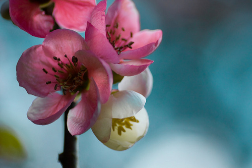
## Reduce the colour used in image with image_quantize.  For example, let's say I want to reduce to 24 colours.
im %>%
  image_resize("500") %>%
  image_quantize(max=24)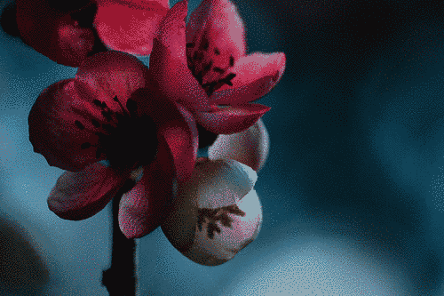
Extracting “Colours” from Quantized Images
I wanted to ulitimately get hex values I can use with ggplot2 to plot, but I got really intrigued with option I can use in image_quantize function. You can specify different colourspace! You can see different colourspaces you can specify by typing in colorspace_types(). There are 37 different colourspaces… I’ve googled bunch… I’ve heard of “HSV”,“RGB”,“Luv”,“CMYK”, but some I have not even heard of before…
## To view different colourspace you can specify in image_quantize function.
colorspace_types()
## [1] "Undefined" "CIELab" "CMY" "CMYK" "Gray"
## [6] "HCL" "HCLp" "HSB" "HSI" "HSL"
## [11] "HSV" "HWB" "Lab" "LCH" "LCHab"
## [16] "LCHuv" "LinearGray" "LMS" "Log" "Luv"
## [21] "OHTA" "Rec601Luma" "Rec601YCbCr" "Rec709Luma" "Rec709YCbCr"
## [26] "RGB" "scRGB" "sRGB" "Transparent" "XYZ"
## [31] "xyY" "YCbCr" "YDbDr" "YCC" "YIQ"
## [36] "YPbPr" "YUV"## Function to get n number of colours out of your image. (optionally you can specify different colour space)
get_colorPal <- function(im, n=8, cs="RGB"){
#print(cs)
tmp <-im %>% image_resize("100") %>%
image_quantize(max=n, colorspace=cs) %>% ## reducing colours! different colorspace gives you different result
magick2cimg() %>% ## I'm converting, becauase I want to use as.data.frame function in imager package.
RGBtoHSV() %>% ## i like sorting colour by hue rather than RGB (red green blue)
as.data.frame(wide="c") %>% #3 making it wide makes it easier to output hex colour
mutate(hex=hsv(rescale(c.1, from=c(0,360)),c.2,c.3),
hue = c.1,
sat = c.2,
value = c.3) %>%
count(hex, hue, sat,value, sort=T) %>%
mutate(colorspace = cs)
return(tmp %>% select(colorspace,hex,hue,sat,value,n)) ## I want data frame as a result.
}
## Here's example using plum flower image
get_colorPal(im)## # A tibble: 8 x 6
## colorspace hex hue sat value n
## <chr> <chr> <dbl> <dbl> <dbl> <int>
## 1 RGB #4D555C 208 0.163 0.361 2501
## 2 RGB #3F8192 192. 0.568 0.573 1108
## 3 RGB #9F717D 344. 0.289 0.624 996
## 4 RGB #6C9BAA 195. 0.365 0.667 590
## 5 RGB #8DB4C2 196. 0.273 0.761 551
## 6 RGB #D36C8D 341. 0.488 0.827 434
## 7 RGB #A5C5D2 197. 0.214 0.824 285
## 8 RGB #CBCCD4 233. 0.0425 0.831 235## if you just want list of colour values...
get_colorPal(im) %>% pull(hex)## [1] "#4D555C" "#3F8192" "#9F717D" "#6C9BAA" "#8DB4C2" "#D36C8D" "#A5C5D2"
## [8] "#CBCCD4"Different Colourspaces and Reduced Colour Palettes
Since using different colourspaces results in slightly different colour sets, I wanted to “map” function in purrr package in action. :)
params <- list(im=list(im),
               n=12, ## number of colour you want
               cs=colorspace_types()[-5]) ## gray fails so I've removed it...

my_colors <- pmap_df(params,get_colorPal)

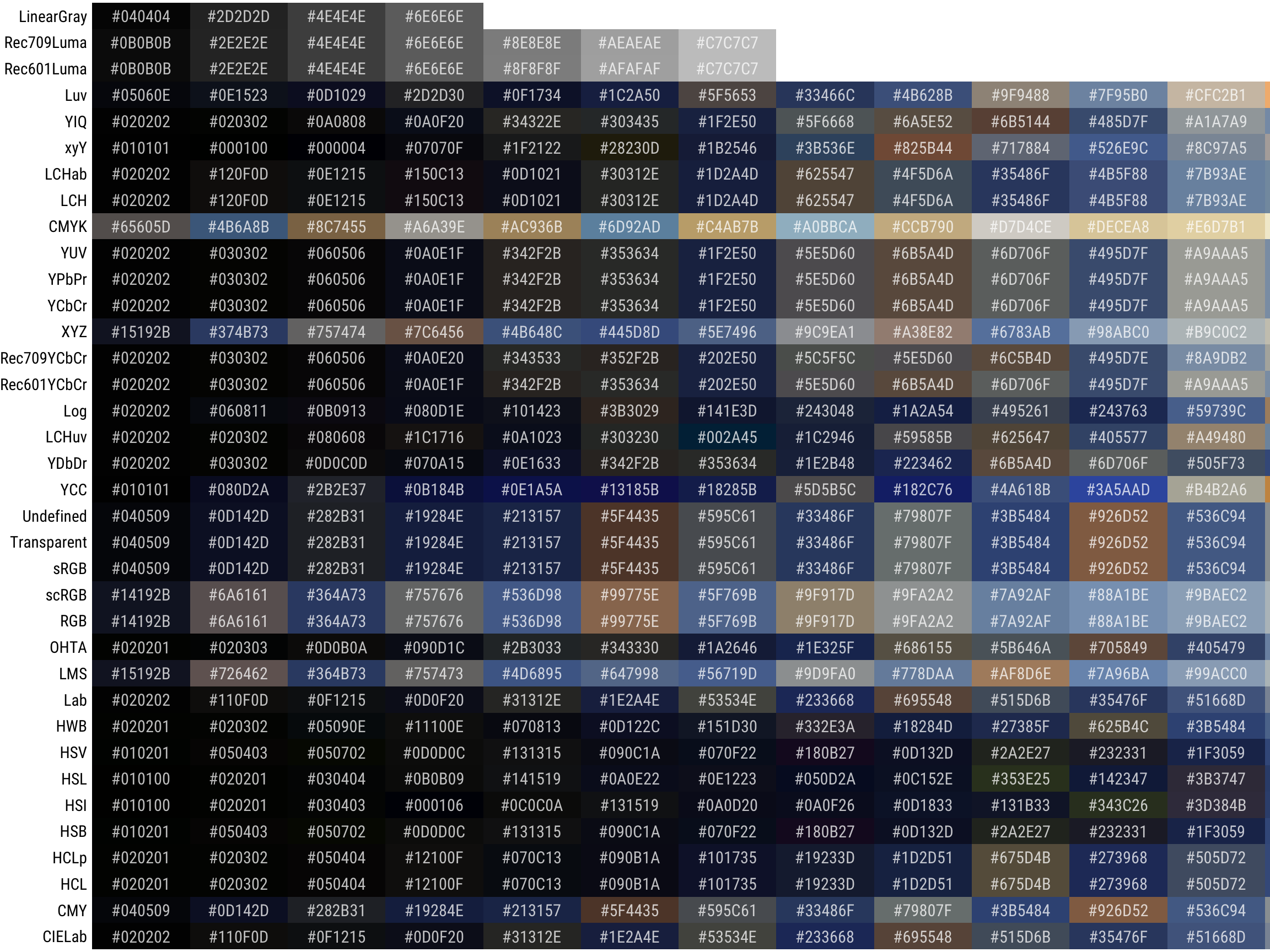
## Let's see what got spitted out as results for different colourspace specifiction in image_quantize function.

## I want to view reduced colours by different colourspaces all at once!
my_colors %>%
  group_by(colorspace) %>%
  mutate(ypos=row_number(value)) %>%  ## I decided to stack colours by value.
  ggplot(aes(x=fct_infreq(colorspace),y=ypos, fill=hex)) +
  geom_tile() +
  geom_text(aes(label=hex), color="#ffffffbe",
            size=4, family="Roboto Condensed") +
  scale_fill_identity() +
  scale_y_continuous(breaks=NULL) +
  theme_void(base_family="Roboto Condensed") +
  coord_flip(ylim=c(1,12)) +
  theme(axis.text = element_text(color = "black", family="Roboto Condensed", hjust=1)) +
  labs(caption="Using different colourspce to reduce the colour used in images")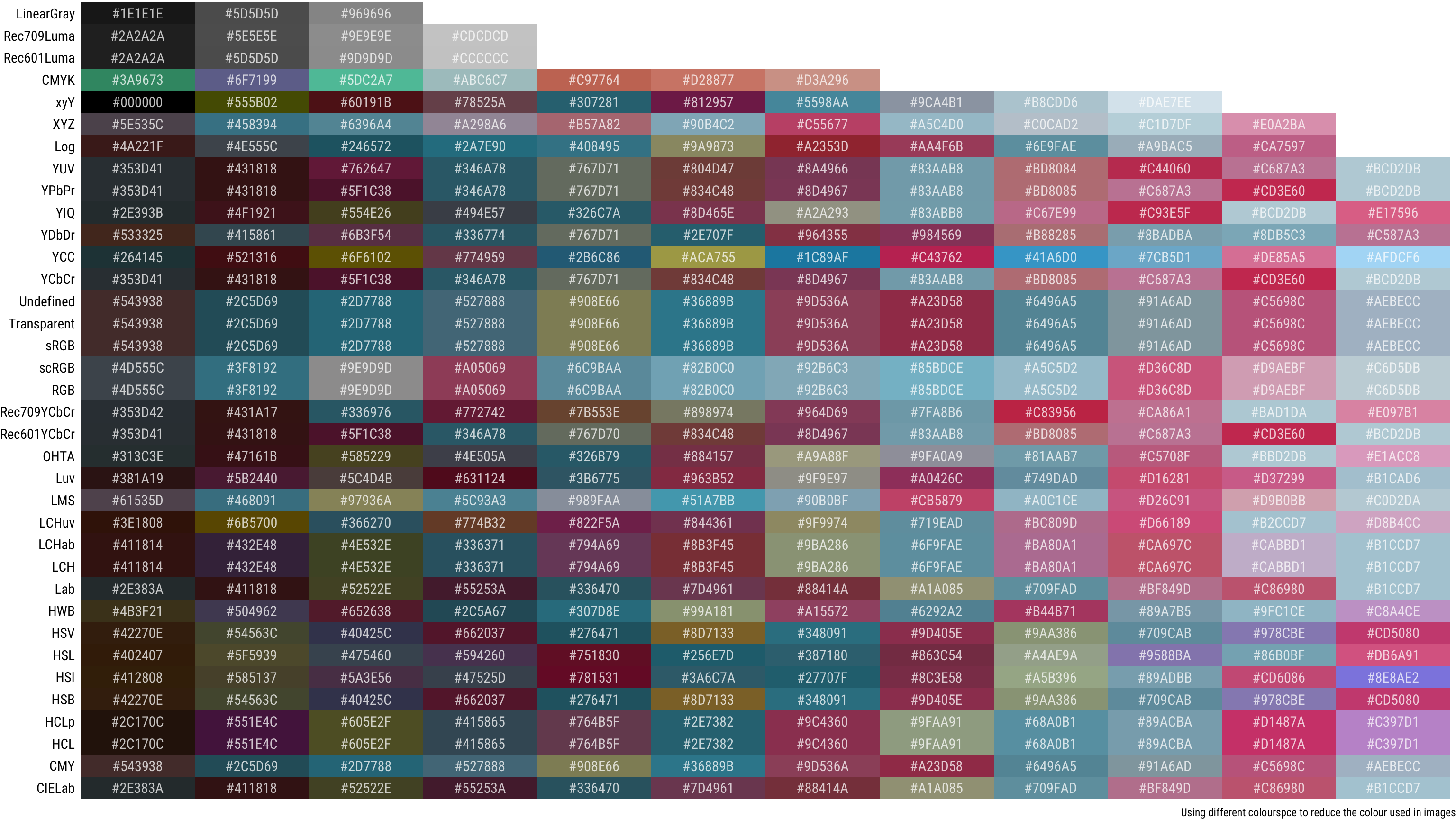
I still don’t undertand why, but some colourspaces returns reduced number of colour palettes below specified max value… I wanted to figure out which colorspaces share same colour palettes, but I wasn’t sure how to go around calculating similarity of palettes…
scRGB and RGB seems to return same results. Also Undefined, Transparent, sRGB seemed to resulted in exact same palettes. LCHab, and LCH in this case was same too. HCLp and HCL are also the same in this case.
Experimenting with plot for fun…
Resulting colour palettes are similar but different… So I’ve decided to play around…
polar1 <-my_colors %>%
  group_by(colorspace) %>%
  mutate(ypos=row_number(hue)) %>%  ## alter stacking order
  ggplot(aes(x=colorspace, y=ypos, fill=hex)) +
  geom_tile() +
  scale_fill_identity() +
  scale_y_continuous(breaks=NULL) +
  theme_void() +
  coord_polar() +
  expand_limits(y=-1)

polar2 <-my_colors %>%
  group_by(colorspace) %>%
  mutate(ypos=row_number(hue)) %>%
  ggplot(aes(x=colorspace, y=hue, fill=hex,
             height=sat*hue, width=value, alpha=value)) +
  geom_tile() +
  scale_fill_identity() +
  scale_y_continuous(breaks=NULL) +
  theme_void() +
  coord_polar() +
  expand_limits(y=0) +
  scale_alpha_continuous(guide="none")

polar3 <-my_colors %>%
  group_by(colorspace) %>%
  mutate(ypos=row_number(hue)) %>%  ## alter stacking order
  ggplot(aes(x=colorspace, y=ypos, fill=hex, height=sat*value)) +
  geom_tile() +
  scale_fill_identity() +
  scale_y_continuous(breaks=NULL) +
  theme_void() +
  coord_polar() +
  expand_limits(y=0)


## I think there's better way to write....
fig_polar <- image_graph(width=600, height=600)
polar1
polar2
polar3
dev.off()
## quartz_off_screen
## 2image_append(fig_polar) ## by default it appends to the side. 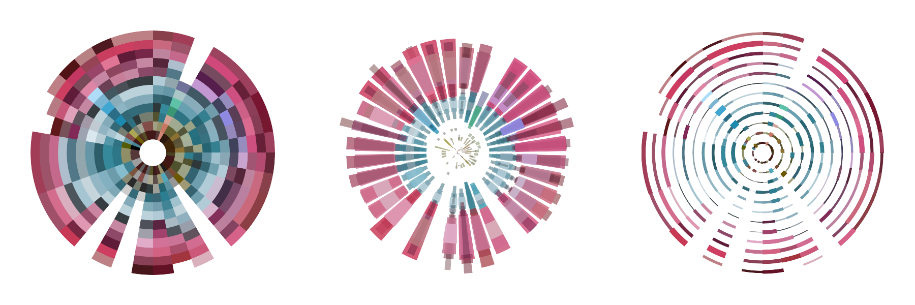
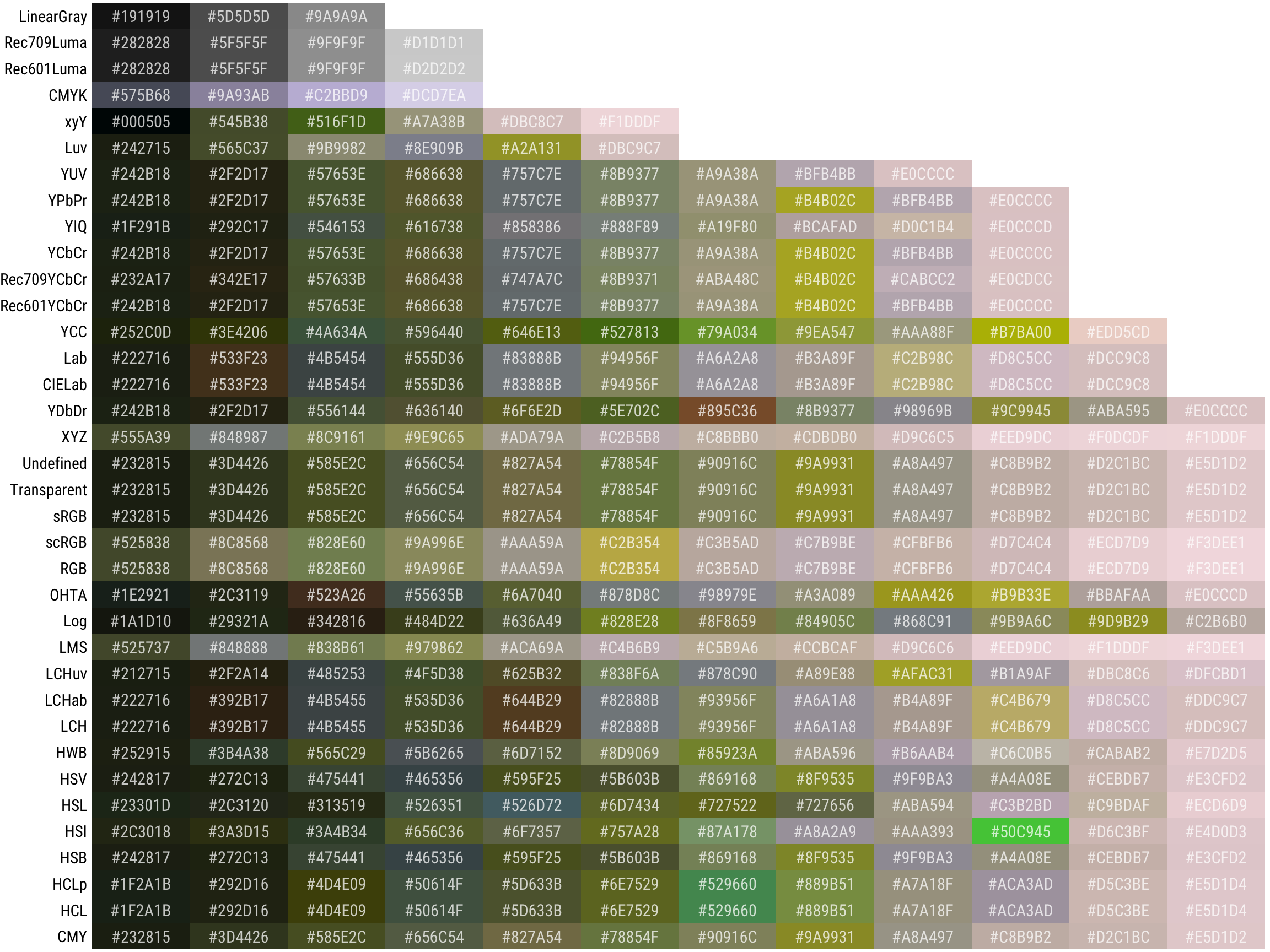
Different Images Differnt Colour Palettes…
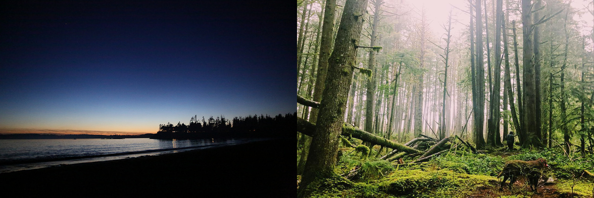
Here are 2 other images I applied same to get colour palettes out of.
## quartz_off_screen
## 2## # A tibble: 1 x 7
## format width height colorspace matte filesize density
## <chr> <int> <int> <chr> <lgl> <int> <chr>
## 1 PNG 1200 600 sRGB TRUE 0 72x72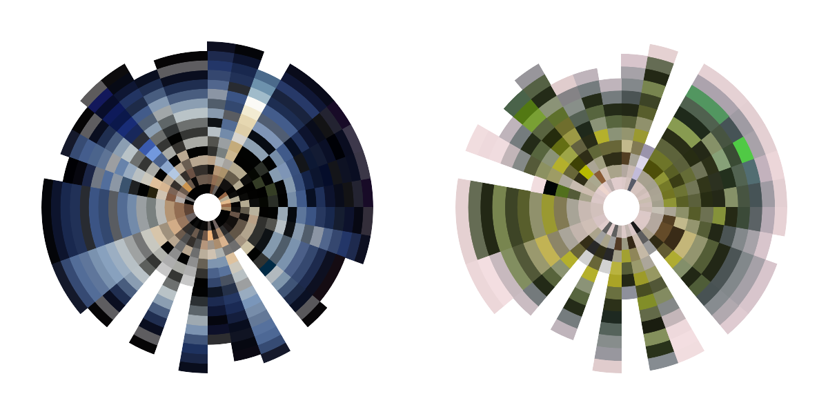

Share this post
Twitter
Google+
Facebook
Reddit
LinkedIn
Pinterest
Email